Ising model on a nearest neighbor random graph 3D

This is another example including Ising model where the underlying graph is a random nearest neighbor graph on plane.

using EasyABM

Step 1: Create Model

In this model we will work solely with the graph and won't need agents. We initially create an empty graph, and then create our model as follows.

graph = dynamic_simple_graph(0) # in a dynamic graph nodes and edges can be added or deleted. 
model = create_graph_model(graph, temp = 2.0, coupl = 2.5, nns = 5, vis_space="3d")

In the initialiser! function we create a list of n = 100 random points in the plane and fill our graph with n nodes and set the position of ith node to the ith random point. We then link each node to its nns number of nearest neighbors and randomly set each node's color to either cl"black" or cl"red" and set spin value to +1 for cl"black" nodes and -1 for cl"red" nodes. In the init_model! function, the argument props_to_record specifies the nodes properties which we want to record during model run.

using NearestNeighbors

const n=100;

vecs = rand(3, n) .* 10
kdtree = KDTree(vecs,leafsize=1)
    
function initialiser!(model)
    flush_graph!(model) # deletes all nodes and edges
    add_nodes!(n, model, color = cl"black", spin =1) # adds n nodes to model's graph with all the nodes having color black and spin 1
    for i in 1:n 
        model.graph.nodesprops[i].pos3 = (vecs[1,i], vecs[2,i], vecs[3,i]) # set positions of nodes in the 3d space
        indices, _ = knn(kdtree, vecs[:,i], model.properties.nns, true) # indices of nearest neighboring vectors
        for j in indices
            if j!=i
                create_edge!(i,j, model)
            end
        end
        if rand()<0.5
            model.graph.nodesprops[i].spin = 1
            model.graph.nodesprops[i].color = cl"black"
        else
            model.graph.nodesprops[i].spin = -1
            model.graph.nodesprops[i].color = cl"red"
        end
    end
end

init_model!(model, initialiser= initialiser!, props_to_record = Dict("nodes"=>Set([:color, :spin])))

draw_graph(model.graph)

Step 3: Defining the step_rule! and running the model

In this step we implement the step logic of the Ising model in the step_rule! function and run the model for 100 steps. At each step of the simulation we take 100 Monte Carlo steps, where in each Monte Carlo step a node is selected at random and its spin and color values are flipped if the Ising energy condition is satisfied.

function step_rule!(model)
    for i in 1:100
        random_node = rand(1:n)
        spin = model.graph.nodesprops[random_node].spin
        nbr_nodes = neighbor_nodes(random_node, model)
        de = 0.0
        for node in nbr_nodes
            nbr_spin = model.graph.nodesprops[node].spin
            de += spin*nbr_spin
        end
        de = 2*model.properties.coupl * de
        if (de < 0) || (rand() < exp(-de/model.properties.temp))
            model.graph.nodesprops[random_node].spin = - spin
            model.graph.nodesprops[random_node].color = spin == -1 ? cl"black" : cl"red"
        end
    end
end

run_model!(model, steps = 100, step_rule = step_rule!)

Step 4: Visualisation

In order to draw the model at a specific frame, say 4th, one can use draw_frame(model, frame = 4). If one wants to see the animation of the model run, it can be done as

animate_sim(model)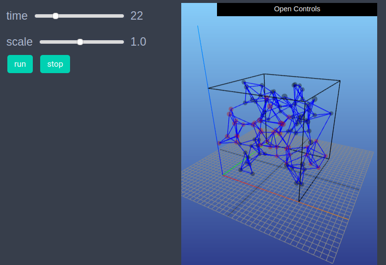

png

After defining the step_rule! function we can also choose to create an interactive application (which currently works in Jupyter with WebIO installation) as shown below. It is recommended to define a fresh model and not initialise it with init_model! or run with run_model! before creating interactive app.

graph = dynamic_simple_graph(0) 

model = create_graph_model(graph, temp = 2.0, coupl = 2.5, nns = 5, vis_space="3d")

create_interactive_app(model, initialiser= initialiser!,
    props_to_record = Dict("nodes"=>Set([:color, :spin])),
    step_rule= step_rule!,
    model_controls=[(:temp, "slider", 0.05:0.05:5.0), 
        (:coupl, "slider", 0.01:0.1:5.0),
        (:nns, "slider", 2:10)],
    node_plots = Dict("magnetisation"=> x -> x.spin),
    frames=100)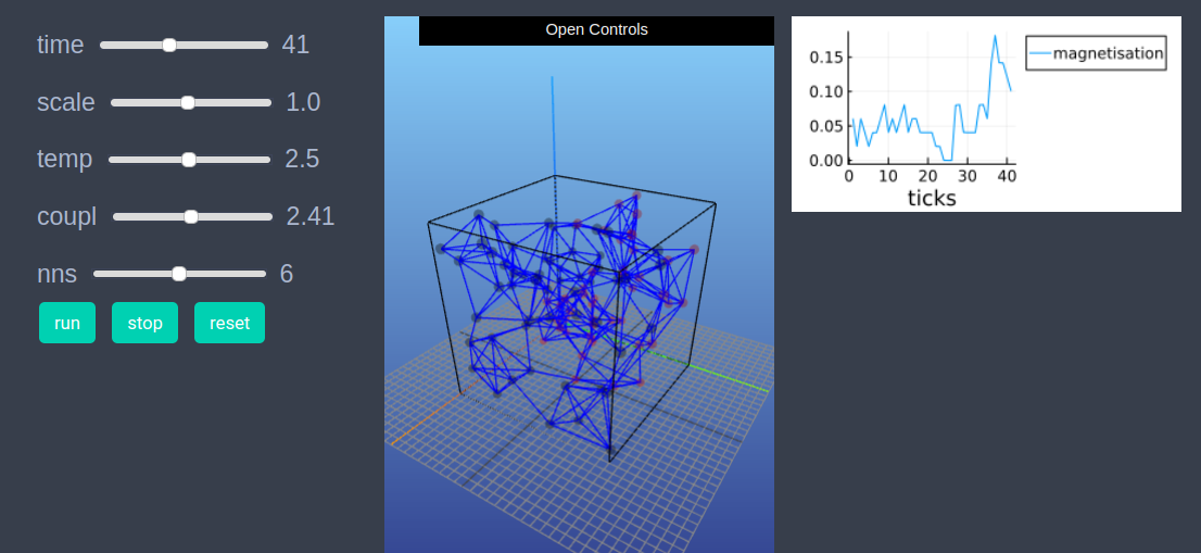

png

Step 4: Fetch Data

In this step we fetch the data of average spin of nodes (also called magnetisation) and plot the result as follows.

df = get_nodes_avg_props(model, node -> node.spin, labels=["magnetisation"], plot_result = true)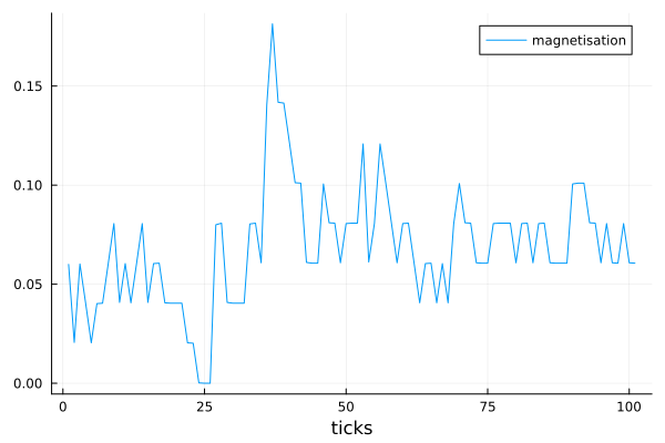

png

References

https://en.wikipedia.org/wiki/Ising_model